Frustratingly Short Attention Spans (ICLR 2017) - A Summary
Through this blogpost I attempt to summarise the key ideas highlighted in an ICLR-2017 accepted paper, Frustratingly Short Attention Spans in Neural Language Modelling, (read it here), by Daniluk et al, of the University College London. You can read the official ICLR reviews on OpenReview.
In my opinion, this is a very well written paper with strongly motivated ideas and strong results. The original manuscript explains the ideas well, and I hope that this blogpost does justice to the paper!
Motivation
This paper is primarily motivated by the shortcomings of the traditional attention mechanism proposed in the Bahdanau et al. ICLR-2015 paper. It tries to improve the traditional attention mechanism with a couple of more meaningful models in the context of language modelling. While implementing their new architecture, the authors notice a strange trend in the lengths of the attention spans (and hence the title) which motivates them to build a simple novel architecture, the “N-Gram Recurrent Neural Network”, which achieves comparable performance to the more complicated attention models.
Hence, this paper ends by questioning the usefulness of complicated attention models, and tries to highlight that today’s state-of-the-art architectures suffer from a long term dependency issue, especially in language modelling.
Traditional Attention Models
The main issue with traditional attention is evident from the equations, they try to squeeze three pieces of information in a single vector. (If you haven’t heard about attention models, you can head over to colah’s blog). As depicted in the figure below, the paper assumes a fixed length attention span.
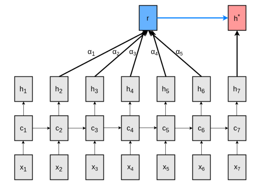
Notation - $x_t$ depicts input vectors, $c_t$ depicts the LSTM hidden vector, $h_t$ depicts the LSTM output vectors, $r$ contains the attention information and $h^*$ represents the final output vector (after attending to previous $h$ units).
Pay close attention to $\color{blue}{h_i}$ in the following equations,
\[\begin{align} \textbf{M}_t & = \tanh(\textbf{W}^Y[\color{blue}{h_{t-L}} ... \color{blue}{h_{t-1}}] + \textbf{W}^h[\color{blue}{h_t} ... \color{blue}{h_t}]) \\ \pmb{\alpha}_t & = softmax(\textbf{w}^T\textbf{M}_t) \\ \textbf{r}_t & = [\color{blue}{h_{t-L}} ... \color{blue}{h_{t-1}}]\pmb{\alpha}^T \\ \textbf{h}^{*}_t & = \tanh(\textbf{W}^r\textbf{r}_t + \textbf{W}^x\color{blue}{h_t}) \end{align}\]In other words,
(Compares each $h_{t-i}$ with $h_t$, using weights $\textbf{W}^{Y}$ and $\textbf{W}^h$)
(Compute attention weights according to previous comparison)
(Weight $h_{t-i}$ according to computed attention weights)
(Compute final vector using attention information and current output vector)
Quite clearly, the output vectors $\color{blue}{h_i}$ are being used in a three-fold role -
- Keys for comparison while computing attention vector.
- Values for computing $\textbf{r}_t$ from attention weights.
- Encode distribution for prediction of next token.
This motivates the key-value and the key-value-prediction model, which attempts to use different vectors (all output vectors of the LSTM) for each of the three roles.
New Attention Models
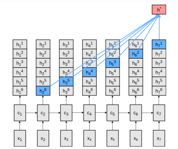
As depicted in Figure 1(b) and 1(c) of the paper, the LSTM produces multiple output vectors (or equivalently, divides $h_t$ into two or more parts). More concretely,
- Key-Value Attention - A different vector is used to compute the attention vector. However, the same vector is still used for the values and predictions.
- Key-Value-Prediction Attention - A different vector is used for each of the three roles described above. More specifically,
The different hidden vector dimensions were chosen to keep identical number of trainable variables. As expected, in nearly all the experiments there is an increasingly better performance from traditional attention, to key-value attention, to key-value-prediction attention. However, the attention visualizations of the model showed a different story.
N-Gram Recurrent Neural Networks
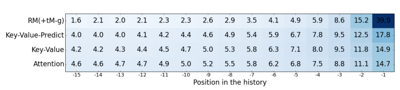
Figure 3(a) and Figure 3(b) of the paper show an interesting trend, and it seems like most of the attention is focussed on the previous 2-5 outputs only. The results of Figure 2(a) show similar perplexities across different attention sizes.
This finding motivates the $N$-Gram RNN, a simple structure which always attends over the previous $N-1$ outputs. This is similar to $N$-gram language models, (Chen and Goodman), which use the previous $N-1$ tokens (a context) to predict the next token. More specifically,
The LSTM outputs $N-1$ vectors (or equivalently divides $\color{blue}{h_{t}}$ into $N-1$ parts, each of which encode information to help predict the $i^{th}$ (from $1$ to $N-1$) token of the future. It’s a very simple neural network, and the four equations in each of the above models are replaced by,
\[\textbf{h}^{*}_{t} = \tanh(\textbf{W}^{N}[\color{blue}{h_{t}^{1}}...\color{red}{h_{t-i+1}^{i}} ... \color{green}{h_{t-N+2}^{N-1} }]^T), i \in \{1, 2, ... N-1\}\]Quite strangely, 4-gram networks perform nearly as well as key-value-predict models (see Figure 2(c)). Of course, this might be very specific to language modelling, but perhaps attention needs a re-thinking?
OpenReview Summaries
This paper received a 7/10 in ICLR-2017 and was accepted for a poster presentation. Here were the major highlights of the reviews -
-
There was some concern about the choice of hyperparameters. The key-value and key-value-predict models were attending over much larger vectors than the traditional models. However, the total number of weights had been adjusted to be uniform across models. There was also some concern over the choice of an attention span of just 15 and an unrolling of just 20 timesteps. The authors do report better results on using BPTT through 35 timesteps.
-
There was a general consensus that an impactful corpus (the Wikipedia corpus) for long-term language modelling had been released, since several dependencies were separated by dozens of timesteps, making it harder for attention based models to capture them.
-
There was a general consensus that a very thorough experimentation was conducted. The paper was well explained and they liked the idea of the $N$-Gram RNN baseline. The paper raises important questions about attention in neural networks.
Clarifications from Authors
I contacted the authors to clarify a few questions raised during the reading group meeting at SLATTIC. Here’s a brief summary of their reply,
- BPTT - There was a concern about the exact mechanism used for Back Propagation Through Time, since the unrolling was done only through a fixed number of timesteps. The input tensors have been broken into chunks of size
batch * bptt_steps * embedding_size, which is used for all gradient calculations in that timestep. After a training step, the final LSTM hidden vectors produced are passed over as the initial hidden vectors for the next training step. (Unless there is a article break). Except this hidden vector, no information about the previous chunks are used during training. Higherbptt_stepsvalues were tried, and produced marginal improvement in results, but the GPU memory constraints limited their experimentation. - Short Attention Spans - Figure 2(a) is a surprising set of results. In the author’s words, “We found that very surprising too. One criticism of our work is that the corpora we trained on might not really need long-range dependencies to learn a good language model – or in other words, cases where such long-range dependencies are really needed are so rare that they don’t provide enough training signal to actually learn a sensible attention mechanism. Check out this thread for the discussion - Twitter.”
Personal Opinions
I personally agree with the comments on OpenReview and the conclusions drawn by the author, and they have done a great job with the explanations in the paper. I’m a bit skeptical about Figure 2(a), since I did not expect such a small variation across attention sizes. A window size of 1 is doing nearly as well as sizes of 5, 10 and 15, which puts a little doubt in my mind about the system. Nevertheless, I think this is great research work since,
-
Raises Important Questions - Instead of trying to beat state-of-the-art, this paper raises an important question - Long term dependencies are far from solved. I think this is a wake-up call for the larger companies that simpler / smarter architectures need to be discovered, and larger / deeper networks aren’t always the solution. The future work sounds really promising, and it would be great to see architectures that force models to ignore local context.
-
Great / Fair Comparisons - I think a good amount of care has been taken to ensure fair comparison between models. The rebuttal on OpenReview supports this.
-
Simpler is Better - Perhaps the part I liked best in this paper is the simplicity of their $N$-gram network idea. This is one of the first papers I’ve seen that tries to match its own model with a baseline model, raising crucial questions.